So we need to tell the model where each token sits. The temptation is to look up how the professionals do it and copy that, but you will understand the real schemes far better if we first try the obvious things and watch them fall over. That is the plan for this chapter. Every failure points directly at the next idea, and by the end we will have arrived at the insight both famous schemes are built on: position as oscillations at different frequencies.
Attempt one: just use the position number
The simplest possible signal: token at position 0 gets the number 0, position 1 gets 1, and so on. To add it to a -dimensional embedding, copy the number across all slots. So the token at position 200 gets a positional vector of , and we add that to its embedding.
It satisfies requirement 1 — different positions get different signals. But it fails requirement 2 spectacularly. Embedding values sit near zero, often between roughly and . A positional value of 200 — or 2000, in a long context — utterly dominates the sum. The token's hard-won meaning is buried under a giant position number. We have told the model where the word is by erasing what it is. Integer encoding is unbounded, and unbounded is fatal.
Attempt two: write the position in binary
The lesson is sharp: keep the values small and bounded. Here is a neat way to bound them — write the position in binary. A position like 200 becomes a row of bits, 11001000, and every entry is now either 0 or 1. Spread those bits across the dimensions and the positional vector lives in the same small range as the embedding. Requirement 2 is satisfied.
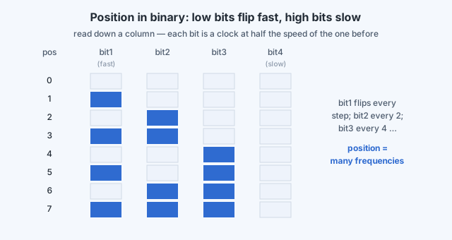
But something far more interesting happens, and it is worth looking at closely. Write out the binary form of consecutive positions and watch each column — each bit position, or index — as you move down the positions:
| position | bit 1 (lowest) | bit 2 | bit 3 | bit 4 |
|---|---|---|---|---|
| 0 | 0 | 0 | 0 | 0 |
| 1 | 1 | 0 | 0 | 0 |
| 2 | 0 | 1 | 0 | 0 |
| 3 | 1 | 1 | 0 | 0 |
| 4 | 0 | 0 | 1 | 0 |
| 5 | 1 | 0 | 1 | 0 |
| 6 | 0 | 1 | 1 | 0 |
| 7 | 1 | 1 | 1 | 0 |
The lowest bit flips every single step — fastest oscillation. The next bit flips every two steps, the next every four, the next every eight. Each index is a clock ticking at half the speed of the one before it.
Low indices oscillate fast across positions; high indices oscillate slowly.
Hold onto that sentence — it is the single most important idea in all of positional encoding. It means a position is pinned down by reading several oscillations at once: the fast bits nail the exact spot, the slow bits say which broad region you are in. It is exactly how a row of clock hands (seconds, minutes, hours) locates a moment in time — the second hand for precision, the hour hand for the big picture.
Why binary still is not good enough
Binary bounded the values and handed us the frequency insight. So why not stop here? Because of requirement 3 and the training process. Those bits are discrete — they jump abruptly between 0 and 1 with nothing in between. Plot any index against position and you get a staircase of sudden jumps, not a smooth curve.
The model's positional patterns are learned during pre-training by gradient descent, and gradients are about smooth, local change — the slope of a function. A staircase of hard jumps has no useful slope; it is flat between jumps and undefined at them. (This is the same reason smooth activations are easier to train than hard steps, back in the Deep Learning course's activation functions lesson.) Abrupt, discontinuous signals make the optimisation harder than it needs to be.
So we have arrived, by elimination, at a precise wish: keep the multi-frequency oscillation idea from binary, but make every signal smooth and continuous instead of a staircase. What function oscillates, is bounded between and , and is perfectly smooth? A sine wave. That single observation is the seed of sinusoidal positional encoding — the subject of the next chapter.
Integer encoding taught us bounded. Binary encoding taught us position = oscillations at many frequencies. Its one flaw was discreteness. Replace the discrete bits with smooth waves of the same graded frequencies and you get sinusoidal encoding; rotate by angles built from those same frequencies and you get RoPE. Everything ahead is this one idea, refined.